CHAPTER 01
Read the labels before turning a valve
The Science Museum's catalogue gives the computer a height of two metres and a weight of 144 kilograms. Its materials include acrylic, metal and rubber. It is large enough for a person to stand beside and complicated enough that a photograph needs some explanation. In its transparent tanks, the quantities being calculated can be watched as they change.
This is one of the hydraulic economic computers associated with Bill Phillips and Walter Newlyn. Their first machine dates from 1949. Later versions acquired the name MONIAC, expanded as Monetary National Income Analogue Computer. The surviving examples are not all identical. A photograph of the prototype and a museum's production machine need not have the same arrangement of pipes. The Science Museum's object record describes one particular survivor.
The labels turn the apparatus into economics. A flow can stand for income, another for consumption, another for taxation. Stored water can represent a balance of money. Adjust a relationship and the flow redistributes. Floats, linkages and shaped pieces help determine what happens next. A result can develop in front of the class instead of appearing as a finished answer beneath an equation.
Before following any particular pipe, ask what its water measures. Litres and litres per minute are different quantities. A tank can remain half full while a great deal of water passes through it. A trickle can eventually fill an empty vessel. Confusing the amount held with the rate of passage will make both the plumbing and the economics unintelligible.
This book begins with the historical machine, then builds several smaller examples you can inspect. The calculations, imaginary transactions and two-tank experiment are original teaching exercises. They do not reproduce the complete MONIAC, and their settings have not been fitted to a country. Their advantage is that you can account for every change without already knowing macroeconomics.
An experiment before the history
Imagine a tank holding ten litres. A tap supplies one litre per minute. An outlet removes one litre per minute. After five minutes, how much water does the tank hold?
Still ten litres, provided the rates stay equal. Five litres have arrived and five have departed. “Nothing happened” would be a poor description of those five minutes, even though the level has not moved.
Now close the outlet for two minutes. Two additional litres accumulate. Open it again at one litre per minute. The level remains at twelve litres; it does not automatically return to ten. To remove the accumulated excess while keeping the tap running, the outlet must temporarily pass more than one litre per minute.
That last sentence contains a small policy problem in a form that can be checked with a measuring jug. Restoring an old rate does not necessarily restore an old amount. Whether the amount recovers depends on how the outlet responds to the level. A fixed outlet and a level-sensitive outlet produce different histories after the same interruption.
We will give the second kind an explicit rule later. For now, leave the answer conditional. The shape of the mechanism matters. It is possible to draw two tanks that look nearly identical and assign them different equations. It is also possible to write the same equation for water, inventory or a queue, while the consequences of applying it to the wrong situation differ considerably.
The attraction of the Phillips–Newlyn machine is partly that it makes such commitments inspectable. A teacher has to arrange a relationship somewhere. An observer can ask what that arrangement means. None of this makes a transparent tank self-explanatory: a clear wall reveals the water, not the reason an economist chose a particular response.
Read the labels, therefore, and keep the units beside them. You will need both when the valves begin to move.
CHAPTER 02
Two names on the machine
Walter Newlyn remembered meeting Phillips among the mature, former-service students at the London School of Economics in 1946. Newlyn studied economics; Phillips was enrolled in sociology, with economics as a subsidiary subject. Their friendship included walks in Surrey and occasional sessions working through problems. Newlyn's recollection is useful because it gives the collaboration a beginning in ordinary student life, rather than presenting the computer as the isolated inspiration of a fully formed professor. His published account opens with those circumstances.
By 1949, Newlyn was teaching at Leeds. The historian Mary Morgan has argued explicitly for restoring his place in the machine's history. Her account describes Phillips's hydraulic ideas, Newlyn's economic blueprint and their joint work on the prototype. The skills were unevenly distributed: Phillips brought more engineering experience; Newlyn brought more economics. Both contributions were needed. Morgan's historical discussion reproduces the blueprint and distinguishes the early machines.
Phillips acknowledged the collaboration at the time. In his 1950 paper, Phillips thanked Newlyn for cooperation, design and construction. He reported that one machine had been made for Leeds and a second, improved version was being built for LSE. The paper did not claim that hydraulics offered the greatest possible precision. Visibility was part of the design requirement.
Doron Swade's later account, written from the museum-conservation side of the story, dates an important LSE demonstration to Lionel Robbins's seminar on 29 November 1949. He also records Leeds support obtained through Newlyn. These details place the apparatus within institutions that could fund, examine and use it. It needed a workshop, materials and people willing to give a student-built machine time in a seminar. Swade's account is also a record of what happened to one of the machines decades later.
What should an inventor get credit for?
There are several jobs concealed inside the phrase “built a model.” Someone chooses the quantities. Someone decides how they relate. Someone finds a physical arrangement that implements those relations. Someone makes the arrangement work reliably enough to demonstrate. Someone explains the result to the people who might otherwise see only an elaborate leak.
The jobs demand different skills. Suppose we want a device to represent household spending. An economist might propose that consumption rises with disposable income, though by less than the full increase. An engineer then needs a way for one measured quantity to move an outlet by a corresponding amount. A machinist needs dimensions and tolerances. A teacher needs a scale the class can read from the back of the room.
The final object cannot tell us, by appearance alone, who contributed each part. That requires documents and testimony. A familiar name engraved on a later exhibit is useful for finding the object; it is not a complete history of its construction.
There is also a temptation to read the finished machine backwards into its makers' lives. Any experience with electricity or money can start to look like preparation for this one invention. The evidence permits a simpler account. Two people with different training worked together on a problem that interested them. They borrowed an analogy, made it more precise and built an apparatus other people could operate.
The prototype supplied a working proposal whose behaviour could be watched, altered and criticized. An improved version could then embody what the first had taught its builders.
We will call it the Phillips–Newlyn machine when discussing the collaboration and MONIAC when referring to the hydraulic computer more generally. Neither name removes the need to identify the particular version when a component, date or restoration is at issue.
CHAPTER 03
The quantity that stays put
A balance is measured at an instant. Income is measured over an interval. If someone says they have five thousand units of currency, you can ask where it is held. If they say they earn five thousand, you need another piece of information: per week, per month or per year?
The missing time unit changes the meaning enormously. In a hydraulic model, the corresponding mistake is to read a tank's litre scale as though it were a flow meter. Both may display the number five. They answer different questions.
Take the original ten-litre tank again. We can describe it with a short rule:
change in stored water = water received − water releasedThis rule applies over an interval. If the incoming rate varies, multiply each rate by the time for which it applies and add the amounts. A constant two litres per minute for three minutes contributes six litres. One litre per minute for the next four minutes contributes four more. The total arrival is ten litres, although the tap was never set to ten litres per minute.
An outlet complicates the arithmetic only by adding another running total. Suppose the tank starts with four litres. It receives six litres in the first interval and releases three. It then receives four and releases six. Its final amount is five litres: four plus six minus three plus four minus six.
You can check that result without knowing what happened within either interval. To know whether the tank overflowed or ran dry along the way, however, you would need the timing. Endpoint bookkeeping can establish the final balance while missing an impossible intermediate state.
An inventory example
Consider an imaginary repair shop with twelve replacement screens in stock. It receives a delivery of eight and fits eleven during the day. Five screens remain at closing. If all eleven customers arrive before the delivery, the original twelve suffice. If it begins with only two, the same daily totals conceal a shortage before the van arrives.
A model that stores only closing inventory can be adequate for a monthly financial report and inadequate for arranging appointments. The relevant time interval comes from the question. There is no universally correct level of detail.
Now suppose the shop reports “twenty screens per week” and “twenty screens in stock” in adjacent spreadsheet cells. Dividing stock by the sales rate gives one week, under an assumption of unchanged sales and no replenishment. Multiplying them gives four hundred screens squared per week, which is probably not the quantity the manager intended. Units are a cheap way to discover a mistaken formula before its output acquires an authoritative-looking chart.
A computer will happily multiply the wrong cells. A physical model can embody the wrong relationship just as faithfully. Its visible movements make some mistakes easier to notice, but the builder still has to interpret them.
Steady does not mean idle
Return to the tank receiving and releasing one litre per minute. The level is steady because two flows balance. Stop both and the level is still steady. A photograph taken at the same level cannot distinguish the working system from the idle one.
A short video might help, but only if the flow is visible. A meter is better. The observation you need depends on the difference you are trying to detect.
We can now describe the system by what it holds, what enters and leaves, and what determines those flows. The first two allow an accounting check. The third allows a prediction. Without an outlet rule, you cannot infer next minute's loss from the present water level.
In the next chapter we will give the outlet such a rule. It is deliberately simple, and its simplicity will let us solve the tank exactly. Keep the repair shop in mind as we do so. A rate proportional to stock may make sense for one process and very little sense for another. A screen does not leave the shelf merely because there are many screens beside it.
CHAPTER 04
A curve cut into plastic
The material in a calculating device can perform mathematical work. In the MONIAC, a shaped template can link an observed quantity to a valve position. Changing the template changes the relationship. The curve has a physical job; it is more than a graph placed beside the machine for explanation.
Allan McRobie's technical account describes a particularly useful component, the Sutro weir. Its shaped opening gives a linear relation between water head and discharge over its intended working range. He also describes plastic graphs, sliders and floats that transmit relationships through the apparatus. His analysis of the machine is worth consulting for the actual arrangements, which are more intricate than the two-tank exercise used here.
This should make us cautious about drawing an ordinary hole at the bottom of a bottle and labelling its output “proportional to volume.” The label alone does not provide that behaviour. A real outlet's discharge depends on its geometry, the water head and conditions of flow. The US Bureau of Reclamation's water-measurement manual treats weir shape and measurement conditions as practical engineering matters.
For our ideal tank, we will specify the rule directly:
outgoing flow = k × stored volumeLet k be 0.2 per minute. Five litres then produce an instantaneous outflow of one litre per minute. Ten litres produce two. The coefficient carries a reciprocal time unit, so multiplying it by litres gives litres per minute.
Emptying is a moving target
If the tank receives no water, it does not lose exactly one litre in the first minute when it starts at five. It begins at that rate, but the rate falls as the tank empties. Under the ideal continuous rule, about 4.094 litres remain after one minute. The loss is about 0.906 litres.
The exact expression is five multiplied by e to the power of minus 0.2 times the elapsed minutes. You do not need to calculate exponentials by hand to see why the curve bends. Every loss reduces the rate of the next loss. Equal time intervals remove equal proportions of what remains, rather than equal volumes.
The time constant is the reciprocal of k. Here it is five minutes. After that interval, the difference from the final equilibrium has fallen to about 36.8 percent of its starting value. After three time constants, roughly five percent remains. “Five-minute response” therefore needs care: five minutes is not the time at which everything has finished.
With a constant inflow of one litre per minute, the equilibrium volume is five litres. Below five, inflow exceeds outflow and the tank fills. Above five, outflow exceeds inflow and it drains. Both movements bring it toward the same level. This is a stable equilibrium in the ideal model.
The shape is a choice
Try a different outlet rule: remove exactly one litre per minute whenever enough water is available. With the same one-litre inflow, every positive level is steady. The system has lost the tendency to return to five litres.
Alternatively, suppose an automatic valve opens fully above six litres and closes below four. The water can repeatedly rise and fall between those limits. That oscillation would come from the switching rule, not from a mysterious property shared by all tanks.
These three devices can be drawn with the same outline. Their behaviour differs because the outlet rule differs. When a historical model produces a cycle or a return to equilibrium, the interesting question is which arrangement causes it.
Software makes changing the rule easy. A physical template makes the chosen rule tangible. In either case, the person presenting the result owes the observer a description of what was installed. We have installed a linear outlet. Everything that follows about our tank depends on it.
CHAPTER 05
The accounts do not choose the answer
One familiar expenditure expression for national output is:
Y = C + I + G + X − MHere C is consumption, I investment, G government purchases of goods and services, X exports and M imports. The categories require definitions. Investment in this account concerns produced capital and inventory, rather than simply the purchase of a financial asset. Buying a share from another investor does not itself manufacture another machine.
Imports are subtracted because spending on foreign production can already appear in the other expenditure components. The subtraction removes that production from the domestic total. It is not a conclusion that every imported item makes the economy poorer. The US Bureau of Economic Analysis explains the expenditure approach with this accounting purpose in view.
Government purchases also differ from the entire government budget. A transfer payment moves income to a recipient; the recipient may subsequently spend it. Counting the transfer as a government purchase and then counting the resulting household purchase would confuse two transactions. BEA's comparison of government-spending measures explains why the larger budget categories are not interchangeable with G.
The imported tool
Use an imaginary, deliberately stripped-down transaction. A workshop imports a tool for 100 currency units and adds it to productive equipment. Ignore transport margins, taxes and every other complication. Investment rises by 100 and imports rise by 100. In the expenditure identity, the two changes offset. The tool was produced abroad.
Now suppose the workshop uses that tool to produce something domestically. That later production is a separate event. The imported tool may be useful to it, but the accounting treatment of the original purchase does not tell us how productive the workshop will become.
BEA gives a related explanation for imported goods entering inventory: the increase can be recorded in both imports and investment in inventories. Its import-and-inventory FAQ addresses the apparent puzzle directly. A person who reads only the minus sign before M may miss the corresponding entry elsewhere.
The lesson for the hydraulic machine is specific. Before treating a diverted stream as a loss, identify the boundary and the account. Water leaving one tank can enter another. A flow leaving the domestic-expenditure circuit can have a counterpart in an external sector. The colour and direction of the pipe do not settle whether a transaction was useful.
An identity needs more instructions
Suppose all you know is that Y equals C plus I, with no government or foreign trade. If I is 20, what is Y?
There is no unique answer. C could be 80 and Y 100. C could be 180 and Y 200. Both satisfy the identity. A program that returns one of them must have received an additional rule, whether its author remembers adding it or not.
Give it the rule C = 0.8Y. Then Y = 0.8Y + 20, so 0.2Y = 20 and Y = 100. The consumption rule selected the answer. The identity ensured that the answer's accounts added up.
Replace 0.8 with 0.6. The same identity now gives Y = 50. Arithmetic has not contradicted itself. We have changed the assumed behaviour.
This distinction helps when someone demonstrates a model by altering a control. “The machine says income falls” is incomplete. Which behavioural rule is installed? Which other quantities have been fixed? How is the model allowed to adjust? Prices, output, borrowing and inventories offer different possible adjustments; a small teaching model may permit only one.
For the next chapter, we will make the assumptions explicit and keep them unchanged long enough to do the calculation. Then we will change one of them. The point is to see exactly where the difference in the answer comes from.
CHAPTER 06
Spending the same unit twice
Imagine a closed economy with no taxes in which every additional unit of income produces 0.75 units of additional consumption. Firms can meet the resulting demand at unchanged prices. Investment is fixed independently of current income. This is an exercise in a small model, not an estimate for an actual economy.
An extra purchase of ten units generates ten units of income somewhere. Recipients spend an additional 7.5. The recipients of that spending spend an additional 5.625. The next increment is 4.21875. Continue the rule and the increments get smaller.
Their sum approaches forty. The first ten has supported a larger total increase in expenditure and income because spending becomes someone else's income and some of that income is spent again.
There is no claim here that a physical ten-unit note has multiplied into four notes. A stock of money and the value of transactions during a period are different quantities. The same means of payment can be used in successive transactions. Chapter three's tank could pass five litres while its level remained unchanged.
Add the series
The calculation is a geometric series:
10 + 10×0.75 + 10×0.75² + … = 10 ÷ (1 − 0.75) = 40The multiplier in this model is four. If the marginal propensity to consume were 0.5, the multiplier would be two. At 0.9, it would be ten. These are consequences of the chosen coefficients and assumptions.
The sequence of rounds is a way of accounting for the repeated response. It does not establish that each round takes a week or that every household waits for the previous round to finish. To make a claim about elapsed time, we would have to add a timing rule. A multiplier can describe a final change while saying nothing about how quickly it arrives.
Now install proportional taxes and imports. Let households consume 0.75 of disposable income, let taxes take 0.2 of income, and let imports rise by 0.1 for each unit of income. Keep other autonomous expenditure at 100 units per period. The equation becomes:
Y = 100 + 0.75×(1 − 0.2)×Y − 0.1×Y
Y = 100 + 0.5×Y
Y = 200
An additional ten units of autonomous expenditure now raises equilibrium Y by twenty. The multiplier is two. Part of each extra income unit does not return as additional demand for domestic production in this simplified circuit.
The words “all else equal” have a bill attached
We held investment fixed. We held the consumption coefficient fixed. We allowed output to respond at unchanged prices. We did not make interest rates rise with the extra activity. We did not give firms a capacity limit or households a reason to revise their behaviour when the policy changed.
Those omissions are useful for isolating the mechanism. They become a problem if we carry the answer into a situation in which the omitted responses matter. A restaurant with empty tables can respond to extra customers differently from one already serving at the limit of its kitchen. A model that has no capacity variable cannot discover that distinction unaided.
Even within our equation, a small change of coefficients can matter. With the consumption propensity at 0.7 rather than 0.75, the denominator becomes 1 minus 0.7 times 0.8 plus 0.1, or 0.54. The multiplier is about 1.85. With consumption at 0.8, it is about 2.17. A tidy integer answer came from tidy chosen numbers.
Before displaying a multiplier, write the denominator in full. It shows which responses have been allowed to reduce or reinforce the initial change. If the evidence for one coefficient is weak, the result should inherit that uncertainty. Printing more decimal places will not repair it.
CHAPTER 07
Two valves moved together
A classroom machine offers an appealing possibility: let different people operate different controls. One adjusts spending, another taxes. The resulting interaction can be instructive, although it can also be hard to attribute. If both controls move between readings, the observer sees their combined effect.
We can first calculate a case in which both changes are precisely specified. Return to the closed economy, remove proportional taxation and imports, and use a lump-sum tax T. Consumption is C₀ plus 0.75 times disposable income. Investment stays fixed. Government purchases are G.
Y = C₀ + 0.75×(Y − T) + I + GRaise G by ten and T by ten. The extra purchases directly add ten to demand. The extra tax reduces consumption by 7.5 under the installed rule. The initial net addition is 2.5. Multiply by four and equilibrium income rises by ten.
This is the balanced-budget result for this particular elementary model. Notice how much care was needed to state it. We switched from a proportional tax to a lump-sum tax. We left imports out. We kept prices, investment and the consumption response fixed. The equality between the final income change and the spending change belongs to that specification.
A prediction you can test on paper
Change the consumption coefficient to 0.6. The initial net demand increase becomes four, because the tax reduces consumption by six. The multiplier becomes 2.5. Four times 2.5 is still ten.
The result does not depend on having chosen 0.75. Algebra shows why: the direct addition is ten times one minus the consumption coefficient, while the multiplier is the reciprocal of one minus that coefficient. The factors cancel.
Now let imports rise with income. The cancellation no longer gives the same answer because an additional term appears in the denominator. The exercise has found a condition under which the result changes. That is more useful than memorizing “balanced budgets have a multiplier of one” without its conditions.
We can also ask about timing. Suppose the purchase happens now and the tax next year. The final static comparison does not describe the intervening path. Households may anticipate the tax, borrowing may change, and production may respond before revenue arrives. Our original equation has no calendar, so it cannot settle these questions.
The saving exercise
There is another small surprise available in the closed model. Let consumption equal 0.8Y and investment equal twenty. Equilibrium income is one hundred. Saving, income minus consumption, is twenty.
Now reduce the consumption share to 0.6 while leaving investment at twenty. Income falls to fifty. Consumption is thirty, and saving is still twenty. The desired saving share rose, but the lower income left the total unchanged.
This example is often used to explain a paradox of thrift. Here you can see every step that produces it. It depends on demand determining output and on investment staying fixed. It does not say that a household should never save, that investment can never respond to financing conditions, or that resources used to build productive capacity are useless.
For an individual household, spending less with income unchanged raises saving. In our aggregate exercise, income is allowed to change because one person's expenditure contributes to another's receipts. Holding household income fixed and holding economy-wide investment fixed are different experiments.
The hydraulic circuit makes this interdependence visible, but the valve settings still need interpretation. A teacher can ask a class to predict the result before making the change, then ask which assumption produced the answer they did not expect. The disagreement becomes more precise once it has a coefficient or a timing rule attached to it.
CHAPTER 08
Let the second tank catch up
Open the two-tank experiment if you would like to operate the example. It starts paused. A holds five litres, B holds ten, and one litre per minute enters from an external source. A releases 0.2 times its volume per minute into B. B releases 0.1 times its volume per minute to an external outlet.
At the starting levels, both outlets pass one litre per minute. Everything balances. The unequal tank volumes are required by the unequal outlet coefficients: B needs twice as much water to produce the same flow.
Double the incoming rate to two litres per minute, then advance one minute at a time. A begins filling immediately. B does not suddenly receive two litres per minute. It receives whatever A's outlet is currently passing, and that outlet responds to A's gradually rising volume.
At the instant of the change, A is still holding five litres. Its outlet still passes one. B's inflow and outflow are therefore still equal at that instant, even though the external supply has doubled. B begins to respond as A accumulates water.
The numbers beneath the drawing
The rules are:
A′ = q − kA×A
B′ = kA×A − kB×B
The prime means rate of change. The incoming flow q is measured in litres per minute. The outlet coefficients kA and kB are measured per minute. A and B are volumes in litres.
For this particular step, with time t measured in minutes from the change, the exact volumes are:
A = 10 − 5×exp(−0.2t)
B = 20 − 20×exp(−0.1t) + 10×exp(−0.2t)
The exponential function appears because each outlet changes continuously with the water level. You can use the table without evaluating the formulas yourself.
| Minutes after the change | A, litres | B, litres | Final outflow, L/min |
|---|---|---|---|
| 0 | 5.00 | 10.00 | 1.00 |
| 5 | 8.16 | 11.55 | 1.15 |
| 10 | 9.32 | 14.00 | 1.40 |
| 20 | 9.91 | 17.48 | 1.75 |
After ten minutes, A has nearly reached its new equilibrium of ten litres. B is still well below its eventual twenty. The last outlet is releasing about 1.4 litres per minute, although the external inflow has been two throughout those ten minutes.
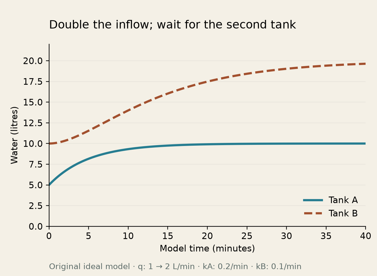
The graph is calculated from the stated equations. It is not a recording from a historical machine. The interactive version uses the same ideal rules and retains the existing water when you change a control.
Where the missing water went
At twenty minutes, total storage is about 27.385 litres, compared with fifteen at the start. Roughly 12.385 additional litres have accumulated. Forty litres arrived over the interval, so about 27.615 litres must have left. The final outflow rate alone would not give that total; it was lower earlier in the run.
This is a useful check on the simulator. We can integrate the outgoing flow independently and compare the result with the storage change. The downloadable workbench performs such checks, along with comparisons against a separate numerical solver. A smooth animation would be insufficient evidence that the calculation was right.
The experiment's time unit is a model minute. During playback, one real second advances one model minute. That speed is for convenience, not a claim about how quickly an economy adjusts. Pressing pause freezes the calculation; a physical tank would need its flows stopped or otherwise controlled.
Try making both outlet coefficients 0.2. The second tank still lags because it receives water through the first. Equal coefficients do not remove the second stage. They give us a useful special case for checking the mathematics, which we will return to when we examine the code.
CHAPTER 09
Correcting yesterday's error
Suppose you are responsible for keeping a tank at ten litres. Its outlet removes a constant one litre per minute while sufficient water remains. You inspect the level once a minute and choose the incoming rate for the next minute. This is a different model from the level-sensitive outlets in the interactive experiment.
At ten litres, set the inflow to one litre per minute. If the tank is below target, add a correction. If it is above, subtract a correction. Write the rule as:
inflow = 1 + g × (10 − observed volume)The coefficient g controls how vigorously you respond. For the one-minute steps used here, a value of 0.5 means correcting half the observed volume error during the next interval, in addition to replacing the litre that will leave.
Start at nine litres. With g equal to 0.5, the first inflow is 1.5 litres per minute. After one minute, the tank holds 9.5 litres. The next inflow is 1.25, leaving 9.75 after another minute. The error halves each time. All rates in this example remain physically possible.
With g equal to one and an exact current reading, the rule corrects the whole error in one step. That sounds attractive. It depends on knowing the current level, delivering precisely the selected flow and knowing the outgoing flow. Remove one of those conditions and the result can change.
A measurement arrives late
Now make the operator use a reading that is one interval old. Set g to one. Suppose the tank was at nine litres at the previous observation and is still at nine when the first correction begins.
The old reading calls for an inflow of two. The tank reaches ten. At the next decision, the available reading is still nine, so the inflow remains two for another minute. The tank reaches eleven. The next available reading is ten, giving inflow one and leaving the tank at eleven. Then the reading of eleven calls for zero inflow, bringing it back to ten. A second old reading of eleven brings it to nine. The pattern repeats.
| Step | Reading used, litres | Inflow for the step, litres/minute | Volume at the end, litres |
|---|---|---|---|
| 1 | 9 | 2 | 10 |
| 2 | 9 | 2 | 11 |
| 3 | 10 | 1 | 11 |
| 4 | 11 | 0 | 10 |
| 5 | 11 | 0 | 9 |
| 6 | 10 | 1 | 9 |
The rule that corrected the error in one step now sustains an oscillation. The water and target have not become unpredictable. The controller is responding to a state the tank has already left.
This example is deliberately exact. Real measurement noise, changing demand and valve limits would alter the sequence. Its purpose is to isolate one delay rather than claim that every delayed controller behaves this way.
Less eager can be more effective
Reduce g to 0.5 while retaining the delayed reading. The corrections are smaller, and the ideal sequence settles toward ten with diminishing swings. The cost is a slower response than the undelayed full correction. We can evaluate that tradeoff because the target, rule and timing have all been specified.
Try writing the first six steps yourself. Use a column for the actual volume and a separate column for the reading available to the operator. Merging those columns accidentally removes the delay and makes the controller look better than it is.
This is why a model of adjustment needs more than a final equilibrium. The route can include overshoot, long waiting periods or repeated corrections. A decision-maker who sees only the latest outcome may intervene before an earlier intervention has finished taking effect.
A hydraulic demonstration can make that waiting visible. A historical economic application still requires evidence about the size and location of its delays. Our six-step tank exercise proves something about its own stated controller; measuring a country's response takes a different kind of work.
CHAPTER 10
A bank is not a bucket of savings
A tank encourages conservation thinking. Water entering one part must come from somewhere, and the total in a sealed circuit cannot increase by changing a label. That physical fact can become a misleading economic assumption if carried over without examination.
Commercial bank lending can create deposits. The Bank of England's 2014 account of money creation explains why banks are not simply passing on deposits that savers previously put aside, and why lending is not a mechanical multiplication of central-bank reserves. Credit creation is constrained by profitability, risk, regulation and monetary conditions. The article by McLeay, Radia and Thomas supplies the institutional explanation.
A hydraulic model can include changes in the amount of water used to represent money. What it cannot do is make the economic interpretation correct merely by conserving its liquid. Before reading a money-stock conclusion from a closed circuit, check whether the model has allowed that stock to change.
Put both sides on the page
Use an imaginary bank and borrower. The bank grants a loan of one thousand currency units and credits the borrower's deposit account by one thousand. Ignore fees, interest and other transactions for this opening entry.
On the bank's side, the loan is an asset: a claim on repayment. The deposit is a liability: an amount owed to the account holder. On the borrower's side, the deposit is an asset and the loan is a liability.
| Participant | Additional asset | Additional liability |
|---|---|---|
| Bank | Loan claim: 1,000 | Customer deposit: 1,000 |
| Borrower | Deposit: 1,000 | Loan owed: 1,000 |
The deposit has increased without an equivalent amount first vanishing from another customer's deposit in this simplified entry. The borrower has not acquired a thousand units of net wealth merely by signing the loan. An obligation has been created alongside the spendable balance.
If the borrower buys equipment, subsequent entries depend on where the seller banks and how the payment settles. A one-bank sketch that omits interbank settlement is inadequate for analyzing an individual bank's liquidity. Adding the missing accounts is necessary before answering that different question.
The Bank of England's shorter money-creation explainer describes deposit creation, deletion on principal repayment and constraints associated with capital and payments to other banks. Its numerical shares describe its publication context; we do not need those dated percentages to understand the entries.
What a drawing leaves out
If you draw the transaction as water moving from “savers” to “borrowers,” you have already chosen a representation. It may help explain one transfer of existing funds. It does not reproduce the opening loan-and-deposit entries above unless additional mechanisms are supplied.
If you draw a tap labelled “new credit,” that alone is also incomplete. You must represent the new obligation, repayment and the conditions under which the tap can operate. Otherwise the drawing has removed the constraints as efficiently as the first drawing removed creation.
The same care applies to the word saving. In the previous chapter's aggregate exercise, saving meant income not consumed during a period. In everyday conversation, “my savings” may mean a stock accumulated over many periods and held in several kinds of assets. A tank label that uses the word without specifying which meaning invites confusion.
There is no requirement that every teaching model contain an entire banking system. A small model can bracket financial details while examining another relationship. The boundary should be visible in its explanation. Someone using it to answer a banking question would then know that additional structure is needed.
For each financial action, identify the counterpart. Who gains an asset? Who acquires a liability? Does the action change a stock, a flow, or both over time? A ledger often answers these questions more efficiently than another pipe.
CHAPTER 11
Four percent of what?
Phillips's 1950 paper discussed keeping the machine's accuracy within about plus or minus four percent through sufficiently precise construction. The surrounding text concerns a calculating apparatus whose physical operations represent equations. It is not a promise that national output can be forecast within four percent. The distinction is visible in the original paper, immediately after Phillips explains his preference for a visible hydraulic demonstration.
A percentage with its object removed travels easily. “Four percent accuracy” is short enough for a caption. The missing object is precisely what determines whether the statement is informative.
Suppose an outlet is intended to deliver one litre per minute at a chosen setting. A measurement finds 0.97. Relative to the intended flow, the difference is three percent. That is a calibration result for that setting and measurement procedure. It says nothing by itself about the other settings, the response during a rapid adjustment, or a forecast made using the outlet as part of a larger model.
Three separate comparisons
First, compare the physical apparatus with its mathematical specification. Does the valve deliver the intended flow? Does the tank scale measure the intended volume? Do the linkages move without excessive friction or slack?
Second, compare the chosen equations with observed behaviour. Does consumption respond in the assumed way under the conditions being studied? Is the delay roughly right? Are the variables measured consistently?
Third, compare a particular forecast with the eventual outcome, using information that was available when the forecast was made. A model fitted after the event has answered a different question from one tested prospectively.
Success at the first comparison does not guarantee success at the second or third. Failure at the first can also spoil an otherwise useful specification. All three deserve separate records.
A calibration table can hide a problem
Imagine testing an outlet at intended flows of 0.5, 1.0 and 1.5 litres per minute. It delivers 0.48, 0.96 and 1.44. Each reading is four percent low. A uniform scale correction might be useful if that proportional error persists across the relevant range.
Now consider readings of 0.45, 1.00 and 1.65. The middle setting is perfect, but the ends differ by minus ten and plus ten percent. Reporting only the central result conceals a shape error. Multiplying every reading by one correction factor will not fix it.
A third outlet may behave differently while opening and closing. At the same marked position, friction or mechanical slack could make the delivered flow depend on the direction of approach. Testing only one direction misses that history dependence.
These are hypothetical measurement examples. They explain what a calibration claim would need to specify: range, method, repeatability and operating conditions. They do not establish the error pattern of any surviving MONIAC.
The wrong equation, perfectly solved
Return to the two-tank experiment. Its numerical solver can agree with the exact solution to many decimal places. Attach the resulting graph to a claim about a real reservoir whose outlet follows a different rule, and those decimals will faithfully describe the wrong system.
You could tune the coefficient so the model matches one observed water level. That fit would be evidence at one condition, not proof that the draining curve has the right shape. Collecting observations at other levels would help discriminate between the possibilities.
A useful report therefore keeps the calculation error and the model discrepancy separate. “The code passed its tests” should identify what the tests establish. In our workbench, they establish agreement with the stated ideal equations and independent numerical checks. They do not certify the historical machine or a country's economy.
A caption repeating the percentage should preserve what was measured. Phillips’s construction claim and a forecast-error claim would require different evidence.
CHAPTER 12
Integration without digits
A tank can accumulate a difference between incoming and outgoing flows continuously. That is an integration operation. Its water level records what has accumulated from the starting condition. No decimal counter is required for the accumulation to occur, although a scale is needed to read it usefully.
Water was not the only physical medium used for this kind of calculation. Vannevar Bush and Harold Hazen's 1931 differential analyzer used mechanical arrangements to solve differential equations. MIT's later reconstruction explains the wheel-and-disc integrator and the torque amplifier that helped transmit its result. The reconstruction's diagrams and animations provide another way to see a mathematical operation implemented in moving parts.
This matters to the chronology. The MONIAC belongs to a history in which several forms of computing coexisted. It was not necessary to wait for water to rescue a world with no other calculating machines. Phillips selected a medium that made particular relationships visible to an audience.
Analogue is a representation
In our hydraulic exercise, volume stands for a continuously varying quantity. In software, a finite numerical representation stores an approximation to that quantity. Both arrangements have limits. The physical apparatus has measurement precision, friction and material behaviour. The digital program has finite arithmetic, a specified algorithm and a display that samples its result.
A physical model is not infinitely accurate because its water level is continuous. You cannot read an unlimited number of reliable digits from a meniscus. A digital model is not automatically inaccurate because it uses discrete numbers. Its numerical error can be made very small relative to the uncertainty in the model's assumptions.
The choice depends on the task. If you want a class to inspect a feedback path, a visible linkage may help. If you want to change hundreds of equations and rerun many parameter combinations, editable code has obvious practical advantages. Those are requirements, not rival claims to being a real computer.
The dangerous large step
We can expose one numerical issue with an emptying tank. Its rule is A′ = −0.2A, starting at five litres. A simple forward-step calculation estimates the next amount by using the current rate for the whole step.
With a one-minute step, it gives five minus one, or four litres. The exact answer is about 4.094. The approximate method has treated the initial outflow as constant even though it should decrease during the minute.
With a ten-minute step, the same method gives five minus ten, or minus five litres. The exact continuous system never contains negative water. The impossible result came from the numerical method and step size, not from the differential equation.
Halving the step repeatedly improves this simple approximation over a fixed interval. More capable methods can achieve greater accuracy with fewer steps. For our two-tank model, an exact constant-setting formula is available, so the browser uses it between control changes.
An animation has its own clock
A screen updates in frames. The calculation need not assume that every frame arrives on schedule. Our experiment measures elapsed real time, converts it to model time and advances the equations. It pauses when the tab is hidden, avoiding a long unseen run when the reader returns.
The graph is sampled at quarter-minute model intervals. Its records therefore do not depend on whether a particular screen happens to refresh more frequently. Changing a slider adds a record at the moment of the change, preserving the settings that belong to the following interval.
These details do not add realism to the economics. They make a small demonstration easier to inspect and reproduce. A CSV row can tell another reader exactly which water volumes and coefficients were present at a particular model time. Someone receiving the picture can check how it was produced.
CHAPTER 13
The other Phillips diagram
Phillips is more often encountered through a curve than through a tank. His 1958 paper examined unemployment and the rate of change of money wage rates in the United Kingdom over 1861–1957. Wage rates were the subject named in its title. Later discussion commonly uses “Phillips curve” for relationships involving price inflation, which can make the original question harder to see.
Wages and consumer prices are related economic quantities, but they are not interchangeable measurements. A worker's wage can rise while the purchasing power of that wage falls. A price index can change because imported energy becomes more expensive, even before a particular worker renegotiates pay.
The Federal Reserve's historical discussion of price stability distinguishes Phillips's original wage-inflation work from subsequent price-inflation analysis and explains the role expectations acquired in the debate. A 2025 lecture by Adriana Kugler likewise treats inflation expectations and supply developments as part of interpreting the relationship. These accounts do not justify a permanent, mechanical menu from which a government can choose any desired combination of inflation and unemployment.
A payslip and a basket
Take a hypothetical hourly wage of twenty currency units. It rises by five percent to twenty-one. Over the same period, the price of a fixed illustrative basket rises by eight percent, from one hundred to one hundred and eight.
The ratio of new to old purchasing power is 1.05 divided by 1.08, or about 0.9722. Purchasing power per hour has fallen by about 2.78 percent. Subtracting eight from five gives a rough minus-three-percent approximation, but the exact ratio is easy to calculate here.
Now reverse the rates: wages rise eight percent and the basket five. The ratio is 1.08 divided by 1.05, about 1.0286. Purchasing power rises about 2.86 percent. The two reversals are not perfectly symmetric because they use different denominators.
This exercise is too small to represent household living standards. Hours worked, taxes, benefits, debt obligations and the household's actual purchases all matter. It distinguishes a nominal wage change from a real purchasing-power change. A chart that silently switches between them changes the question.
A fitted line is not a control knob
Suppose a scatter plot shows lower unemployment in years with faster wage growth. That observation can motivate a theory. It does not, by itself, identify what would happen if a policymaker deliberately altered one variable while everything else responded.
An experiment on the two-tank simulator is different. We know the incoming flow was changed because we changed it, and we know the other coefficients because we set them. The program contains no hidden wage bargain, import-price shock or revision to expectations. Historical economic data arrive without that degree of control.
Even the definition of the measured population matters. An average wage can change because the wages of the same workers change, because the mix of workers changes, or both. To see the arithmetic, imagine two equally sized groups earning ten and thirty. Their average is twenty. If the lower-paid group leaves the measured sample while the higher-paid group's wage stays unchanged, the observed average rises to thirty without either group's wage rate increasing.
No particular labour-market release is being described here. It shows why a plotted aggregate needs a measurement description. The apparent movement can have more than one source.
Phillips's empirical paper and the hydraulic machine ask related but distinct questions. The apparatus lets specified relationships generate a path. Empirical work examines whether proposed relationships describe observations. Moving successfully between the two requires measurement and argument, rather than a confidence that the same surname makes the connection automatic.
If you encounter a Phillips-curve chart, begin with its axes. Is the vertical variable wage growth, price inflation or something else? What period and population are represented? Are expectations included? Those questions will tell you more than trying to decide, from the title alone, whether “the curve” has finally been proved or disproved.
CHAPTER 14
To run it or preserve it
A working hydraulic computer is also a collection of ageing materials. Pumps corrode, seals deteriorate and transparent surfaces can become difficult to read. Restoring operation may require replacement parts. Preserving the object may require leaving it dry.
The Reserve Bank of New Zealand's 2007 account records several stages in the history of its displayed machine: transfer from LSE to the New Zealand Institute of Economic Research in 1987, restoration in 1991, later refurbishment and further work before museum display in 2007. It mentions pump corrosion and the need to reseal tanks. The same article states that the MONIAC was not used for the Bank's policy analysis. The institutional report separates a working educational exhibit from the machinery used for actual policy modelling.
Swade's 1995 conservation account describes a different choice for the Science Museum example. Following its last operation in May 1992, conservation involved roughly two hundred hours of work. Keeping a machine available as an historical object can justify decisions different from those needed to run a demonstration. LSE's 2016 account of the museum display describes a non-operating machine accompanied by an interactive virtual version.
Cambridge's Marshall Library archive page lists its restored machine and related materials, including demonstration resources. The Reserve Bank's MONIAC resource page offers another recorded explanation. A video can show a machine operating at a documented time without requiring us to claim that every surviving example is working today.
What would you replace?
Imagine an old teaching apparatus with a failed pump. A modern replacement can deliver the correct flow but looks different and sounds quieter. Installing it restores the calculation while changing the historical assembly. Leaving the original preserves the component while preventing operation. Keeping both, with the replacement identified, may serve another purpose.
There is no single answer independent of the collection's aim. A museum preserving manufacturing evidence and a teaching laboratory demonstrating flow equations may reasonably make different decisions. What would be misleading is to replace the component and leave the visitor unaware of the change.
The same issue arises with a template. Suppose its original curve is damaged and a new one is cut from an old drawing. The reconstructed relationship depends on the drawing's scale and interpretation. A neat replacement may work better than the surviving part while introducing uncertainty about the original settings.
A restoration record should therefore say what was retained, repaired, replaced or inferred. Photographs of the finished object are not enough. The work that makes an exhibit convincing can also remove the evidence of how much reconstruction was necessary.
Software has a restoration problem too
Our small browser model avoids pump corrosion, but its future operation is not guaranteed merely because the files are digital. Browsers change. A hosting service can disappear. An external dependency can become unavailable. An undocumented numerical convention can be forgotten.
For that reason, the companion is available as a small source archive with no framework or remote library requirement. The equations, initial conditions and tests are included. Another person can inspect or reimplement it without obtaining an account or contacting the original site.
That choice preserves the specification more effectively than a screen recording alone. The recording would show what one run looked like; the source and equations explain how to produce other runs. Conversely, a recording of the historical MONIAC can preserve mechanical behaviour that our simplified source does not attempt to represent.
A collection can preserve several forms of evidence: the object, drawings, operating notes, films, measurements and code for later interpretations. Each retains something the others omit. When you follow the museum links, notice which kind of evidence you are being shown. A restored demonstration shows operation; an original photograph records an earlier state; a new simulation exposes a later interpretation.
CHAPTER 15
A calculation you can take apart
The downloadable workbench contains the original two-tank calculation, the browser interface and an independent numerical checker. You can open the page locally. The calculation itself is short enough to read without knowing the rest of the website.
Its central function accepts six numbers: the two current volumes, incoming flow, two outlet coefficients and the amount of time to advance. It returns the next two volumes. All other features—sliders, drawing, graph and CSV export—use that result.
This separation gives us a useful place to test. If the drawing is wrong, we can inspect the returned numbers. If the numbers are wrong, changing the colour or frame rate will not help.
Start with the first tank
With constant q and kA, tank A approaches q divided by kA. Call its starting volume A₀. Its volume after time t is:
A(t) = q/kA + (A₀ − q/kA) × exp(−kA×t)The first term is the equilibrium. The second is the starting deviation multiplied by a decaying factor. At t equal to zero, the factor is one and the expression returns A₀. At very large t, the factor approaches zero and the equilibrium remains.
These two endpoint checks are simple enough to perform before trusting any code. They catch a surprising number of sign and initialization mistakes.
Tank B receives A's changing outflow. Its solution includes both exponential rates. When the rates differ, one part contains a ratio whose denominator is kB minus kA. That looks troublesome when the rates are equal, but the physical model has no singularity at that setting. The ratio has a finite limit.
With both rates equal to k, the second tank's expression is:
B(t) = q/k + (B₀ − q/k)×exp(−k×t)
       + k×(A₀ − q/k)×t×exp(−k×t)
A program that simply divides by the difference between equal coefficients would fail at an entirely ordinary slider setting. The implementation handles the equal-rate limit and uses a numerically stable form when the rates are close.
Test a different route to the answer
Copying the same closed-form equation into a test can repeat the same mistake. The checker therefore compares the JavaScript result with a separately implemented fourth-order Runge–Kutta integration of the two differential equations. That method advances through small time steps rather than evaluating the closed-form solution.
The checks cover 110 selected and reproducibly randomized cases. They include zero inflow, equilibrium, equal and nearly equal outlet rates, different starting volumes and long intervals. Additional checks integrate the outgoing flow and compare it with incoming water and the change in storage.
Agreement within the stated numerical tolerance is evidence that these implementations solve the same ideal equations. It is still possible for both to be based on an inappropriate model of a real apparatus. Testing the calculation and validating an application remain separate jobs.
Read the exported file
The CSV begins with time, the two volumes, incoming flow and the two outlet coefficients. Those columns are sufficient to restart a constant-setting interval. Choose a row, supply its volumes and coefficients to the calculation, and advance by the difference between its time and the next row's time. The result should agree with the next recorded volumes within rounding, provided no unrecorded setting change occurred.
Two rows can share a timestamp when a slider moves while the model is paused. Their volumes should match even if a coefficient differs. Treat the later row's settings as the ones that apply afterward. Averaging the two coefficients would invent an interval that never happened.
To compare two runs fairly, choose the same model times rather than the same row numbers. One run may contain extra rows documenting adjustments. A spreadsheet chart that spaces every row equally would then distort elapsed time. Use the time column as a numerical horizontal axis, and keep the units on the exported figure.
A small bug with a plausible picture
Imagine writing B's incoming flow as kA times B rather than kA times A. The variable names are similar, and both expressions produce a number with the right units. The program might still draw a smooth curve.
The steady-state test would expose the mistake at the default settings. With A equal to five, B equal to ten, kA equal to 0.2 and kB equal to 0.1, the incorrect B equation gives an incoming flow of two and outgoing flow of one. B would rise even though the intended system begins at equilibrium.
A conservation check would also help: the flow leaving A would no longer equal the flow entering B. The system would create or lose water at the connection. The test catches the error by checking the connection between the tanks. It does not need a preferred graph to compare against.
If you modify the model, keep the tests that still describe its intended behaviour and change the ones whose assumptions you deliberately replaced. Record the new rule in the page itself. A fork with a nonlinear outlet or feedback controller can be an interesting experiment, provided its reader can discover what has changed.
CHAPTER 16
Five runs worth keeping
A model becomes easier to understand when you make a prediction before pressing Play. Keep the first prediction, including the wrong parts. Otherwise a smooth result can make you feel that you expected it all along.
The following runs use the original two-tank companion. Reset before each one unless instructed otherwise. The displayed coefficients are per minute, the incoming flow is litres per minute, and the volumes are litres. No historical machine settings are implied.
One: change the inflow, keep the outlets
Set incoming water to two while leaving A's coefficient at 0.2 and B's at 0.1. Predict the final levels and which tank moves first. The equilibrium equations give A equal to ten and B equal to twenty. The early path is in chapter eight.
Advance five minutes and save the values. Advance another five and compare. A's second five-minute gain is smaller than its first. B's gain over the second interval is larger than over its first, because its incoming flow has had time to rise. The two curves have different early shapes even though both eventually settle.
Two: open A's outlet
Reset, keep incoming water at one, and raise A's coefficient to 0.4. A's initial outflow doubles from one to two, so A begins draining and B begins filling. The new equilibrium for A is 2.5 litres. B's eventual equilibrium is still ten, because the unchanged external supply must eventually pass through its unchanged outlet.
B therefore rises temporarily and later returns toward its starting level. A single before-and-after comparison would miss that excursion. Export the run and find the largest recorded B value. The quarter-minute sample may lie slightly below the exact continuous peak, so report it as the largest sampled value.
Three: open B's outlet
Reset and raise B's coefficient to 0.2. B begins draining toward five litres. A stays at five, because our one-way model gives B no influence over A. If your intuition expected A to respond, identify the missing physical connection that would be required.
In a real arrangement, downstream pressure or a shared mechanism might create such a connection. Our ideal open transfer does not include one. Adding it would require another relationship, rather than simply relabelling the same equations.
Four: stop the incoming water
Reset and set incoming water to zero. Both tanks ultimately empty under the ideal rules, approaching zero continuously. A starts falling immediately. B's rate of change is initially zero because A's initial outflow still equals B's. B then falls as A supplies less.
Track the total remaining water rather than either tank alone. With no incoming water, it can only decrease. If a modified program makes the total increase during this run, inspect the connection and signs before interpreting the curve.
The exact mathematical volumes approach zero without reaching it at a finite time. A real tank eventually encounters effects excluded by the ideal proportional rule, and a displayed value rounds to 0.00 long before proving exact emptiness. The display precision should not be mistaken for a physical threshold.
Five: make a pulse
Reset, set inflow to two, advance five minutes, then restore inflow to one. Keep the outlet coefficients unchanged. The external tap is back at its original setting, but the tanks contain extra water. B can continue rising for a while after the tap has been turned down because A is still releasing more than its original one litre per minute.
Record the time at which B reaches its largest sampled value. Compare it with the five-minute moment when the pulse ended. This is a compact example of why an outcome can keep changing after its original input has stopped changing.
On the quarter-minute recording grid, B reaches about 12.449 litres at 9.75 minutes in this pulse experiment. That is nearly five minutes after the incoming rate was restored. For the second run, opening A’s outlet, the largest sampled B volume is about 11.574 litres at 4.5 minutes. These values provide checks on your exported rows.
If you share a run, include the initial conditions and the timing of each adjustment. “I turned the water up and B rose later” is an observation; the settings make it reproducible. The CSV preserves those details, including repeated timestamps when a setting changes without intervening model time.
The historical machine offered a roomful of people this kind of shared object to argue over. Our smaller version gives you enough controls to pose a question and enough arithmetic to check the answer. Choose one of the runs, write down what you expect, and let the second tank take its time.
Sources & edition note
First full edition: sixteen chapters, original worked examples and an interactive two-tank companion with downloadable source and independent numerical checks. Historical reporting is distinguished from the book’s hypothetical exercises.
Ada Vale is a fictional editorial pen name. This book was researched and written with AI assistance; sources and original calculations are provided for inspection.
- The Science Museum's object record ↗
Object record for a particular surviving hydraulic computer; dimensions and materials, rather than a universal specification for every machine.
- His published account ↗
Walter Newlyn’s first-person chapter (2000); publisher’s opening excerpt consulted, not the inaccessible full chapter.
- Morgan's historical discussion ↗
Mary Morgan (2014), historical evidence for Newlyn’s contribution and the early prototype; original essay and reproduced archival drawings.
- Swade's account ↗
Doron Swade (1995), curator’s record of the 1949 demonstration and later conservation.
- His analysis of the machine ↗
Allan McRobie (2011), author’s technical paper on components and specific business-cycle experiments; consulted full text.
- Water-measurement manual ↗
US Bureau of Reclamation, weir geometry and operating conditions.
- US Bureau of Economic Analysis explains the expenditure approach ↗
BEA (2025), GDP accounting and the treatment of imports.
- Comparison of government-spending measures ↗
BEA, distinction between purchases included in GDP and wider expenditure measures.
- Its import-and-inventory FAQ ↗
BEA, offsetting entries for imported goods added to inventory.
- The article by McLeay, Radia and Thomas ↗
Bank of England (2014), commercial-bank deposit creation and its constraints.
- Money-creation explainer ↗
Bank of England (2019), introductory loan/deposit and repayment explanation.
- The original paper ↗
A. W. Phillips (1950), Mechanical Models in Economic Dynamics. Original scanned pages inspected; visibility, Newlyn’s collaboration and the construction-accuracy claim.
- The reconstruction's diagrams and animations ↗
MIT wheel-and-disc differential-analyzer reconstruction and original Bush–Hazen paper references.
- Historical discussion of price stability ↗
Ben Bernanke (2006), historical distinction between wage and price inflation and the expectations debate.
- 2025 lecture by Adriana Kugler ↗
Adriana Kugler (2025), interpretation of Phillips curves with expectations and supply developments; dated speech, not current policy advice.
- The institutional report ↗
Ng and Wright, RBNZ Bulletin 70(4), 2007, restoration record and explicit distinction from actual policy analysis.
- 2016 account of the museum display ↗
LSE (2016), Science Museum display with a non-operating object and virtual companion.
- Marshall Library archive page ↗
Cambridge Marshall Library, machine-related archive and demonstration resources.
- Reserve Bank's MONIAC resource page ↗
Reserve Bank of New Zealand, recorded demonstration and transcript published December 2024.